Grid Point Projection

In ECoG datasets the electrode locations are usually different. For this reason, we established a grid with a set of points defined in a standardized MNI brain. Data is then interpolated to this grid, such that they are common across patients, which allows across patient decoding use cases.

In this notebook, we will plot these grid points and see how the features extracted from our data can be projected into this grid space.

In order to do so, we’ll read saved features that were computed in the ECoG movement notebook. Please note that in order to do so, when running the feature estimation, the settings

Note

stream.settings['postprocessing']['project_cortex'] = True
stream.settings['postprocessing']['project_subcortex'] = True

need to be set to True for a cortical and/or subcortical projection.

import numpy as np
import matplotlib.pyplot as plt

import py_neuromodulation as nm

Read features from BIDS data

We first estimate features, with the grid_point projection settings enabled for cortex.

RUN_NAME, PATH_RUN, PATH_BIDS, PATH_OUT, datatype = nm.io.get_paths_example_data()

(
    raw,
    data,
    sfreq,
    line_noise,
    coord_list,
    coord_names,
) = nm.io.read_BIDS_data(PATH_RUN=PATH_RUN)

settings = nm.NMSettings.get_fast_compute()

settings.postprocessing.project_cortex = True

channels = nm.utils.set_channels(
    ch_names=raw.ch_names,
    ch_types=raw.get_channel_types(),
    reference="default",
    bads=raw.info["bads"],
    new_names="default",
    used_types=("ecog", "dbs", "seeg"),
    target_keywords=["MOV_RIGHT_CLEAN", "MOV_LEFT_CLEAN"],
)

stream = nm.Stream(
    sfreq=sfreq,
    channels=channels,
    settings=settings,
    line_noise=line_noise,
    coord_list=coord_list,
    coord_names=coord_names,
    verbose=True,
)

features = stream.run(
    data=data[:, : int(sfreq * 5)],
    out_dir=PATH_OUT,
    experiment_name=RUN_NAME,
    save_csv=True,
)

Extracting parameters from /opt/hostedtoolcache/Python/3.11.10/x64/lib/python3.11/site-packages/py_neuromodulation/data/sub-testsub/ses-EphysMedOff/ieeg/sub-testsub_ses-EphysMedOff_task-gripforce_run-0_ieeg.vhdr...
Setting channel info structure...
/opt/hostedtoolcache/Python/3.11.10/x64/lib/python3.11/site-packages/py_neuromodulation/utils/io.py:61: RuntimeWarning: Did not find any events.tsv associated with sub-testsub_ses-EphysMedOff_task-gripforce_run-0.

The search_str was "/opt/hostedtoolcache/Python/3.11.10/x64/lib/python3.11/site-packages/py_neuromodulation/data/sub-testsub/**/ieeg/sub-testsub_ses-EphysMedOff*events.tsv"
  raw_arr = read_raw_bids(bids_path)
Reading channel info from /opt/hostedtoolcache/Python/3.11.10/x64/lib/python3.11/site-packages/py_neuromodulation/data/sub-testsub/ses-EphysMedOff/ieeg/sub-testsub_ses-EphysMedOff_task-gripforce_run-0_channels.tsv.
/opt/hostedtoolcache/Python/3.11.10/x64/lib/python3.11/site-packages/py_neuromodulation/utils/io.py:61: RuntimeWarning: The unit for channel(s) MOV_RIGHT has changed from V to NA.
  raw_arr = read_raw_bids(bids_path)
/opt/hostedtoolcache/Python/3.11.10/x64/lib/python3.11/site-packages/py_neuromodulation/utils/io.py:61: RuntimeWarning: Other is not an MNE-Python coordinate frame for IEEG data and so will be set to 'unknown'
  raw_arr = read_raw_bids(bids_path)
Reading electrode coords from /opt/hostedtoolcache/Python/3.11.10/x64/lib/python3.11/site-packages/py_neuromodulation/data/sub-testsub/ses-EphysMedOff/ieeg/sub-testsub_ses-EphysMedOff_space-mni_electrodes.tsv.
/opt/hostedtoolcache/Python/3.11.10/x64/lib/python3.11/site-packages/py_neuromodulation/utils/io.py:61: RuntimeWarning: There are channels without locations (n/a) that are not marked as bad: ['MOV_RIGHT']
  raw_arr = read_raw_bids(bids_path)
/opt/hostedtoolcache/Python/3.11.10/x64/lib/python3.11/site-packages/py_neuromodulation/utils/io.py:61: RuntimeWarning: Not setting position of 1 misc channel found in montage:
['MOV_RIGHT']
Consider setting the channel types to be of EEG/sEEG/ECoG/DBS/fNIRS using inst.set_channel_types before calling inst.set_montage, or omit these channels when creating your montage.
  raw_arr = read_raw_bids(bids_path)

From analysis.py, we use the :class:~`analysis.FeatureReader` class to load the data.

# init analyzer
feature_reader = nm.FeatureReader(feature_dir=PATH_OUT, feature_file=RUN_NAME)

To perform the grid projection, for all computed features we check for every grid point if there is any electrode channel within the spatial range `max_dist_mm`, and weight this electrode contact by the inverse distance and normalize across all electrode distances within the maximum distance range. This gives us a projection matrix that we can apply to streamed data, to transform the feature-channel matrix (n_features, n_channels) into the grid point matrix (n_features, n_gridpoints).

To save computation time, this projection matrix is precomputed before the real time run computation. The cortical grid is stored in py_neuromodulation/grid_cortex.tsv and the electrodes coordinates are stored in _space-mni_electrodes.tsv in a BIDS dataset.

Note

One remark is that our cortical and subcortical grids are defined for the left hemisphere of the brain and, therefore, electrode contacts are mapped to the left hemisphere.

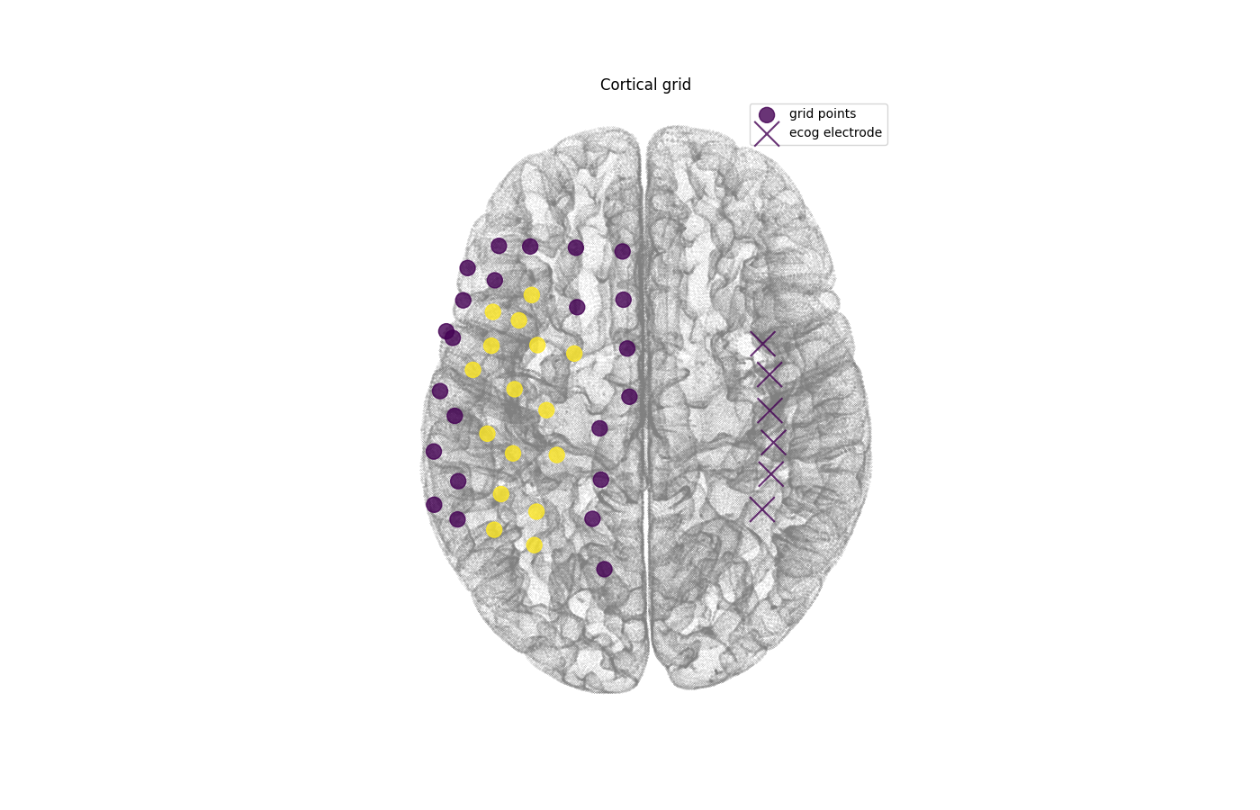
From the analyzer, the user can plot the cortical projection with the function below, display the grid points and ECoG electrodes are crosses. The yellow grid points are the ones that are active for that specific ECoG electrode location. The inactive grid points are shown in purple.

feature_reader.plot_cort_projection()

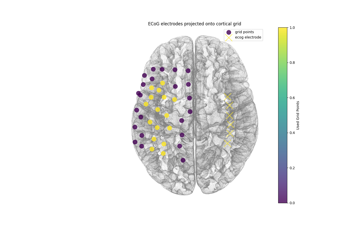
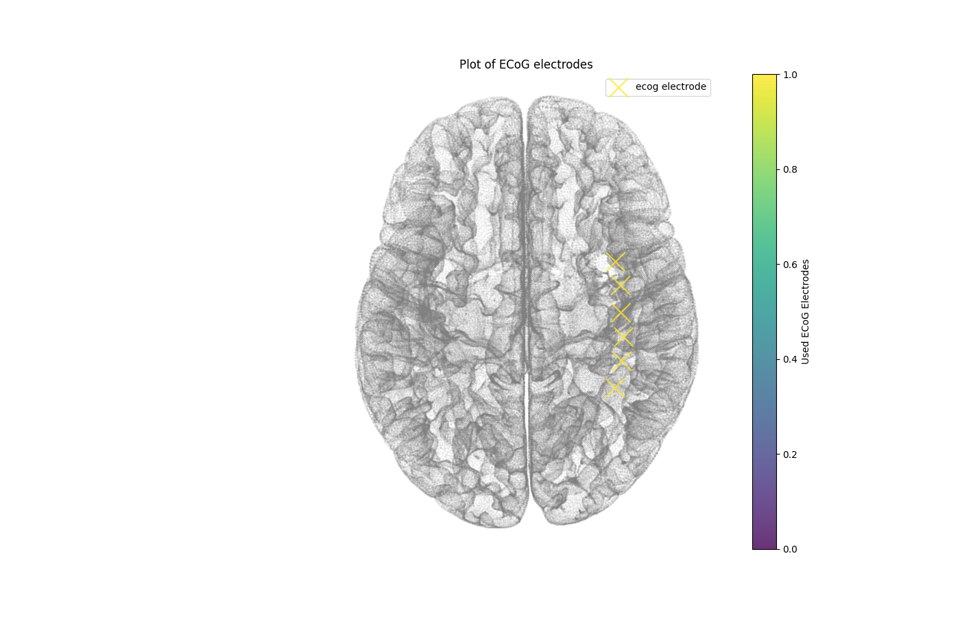
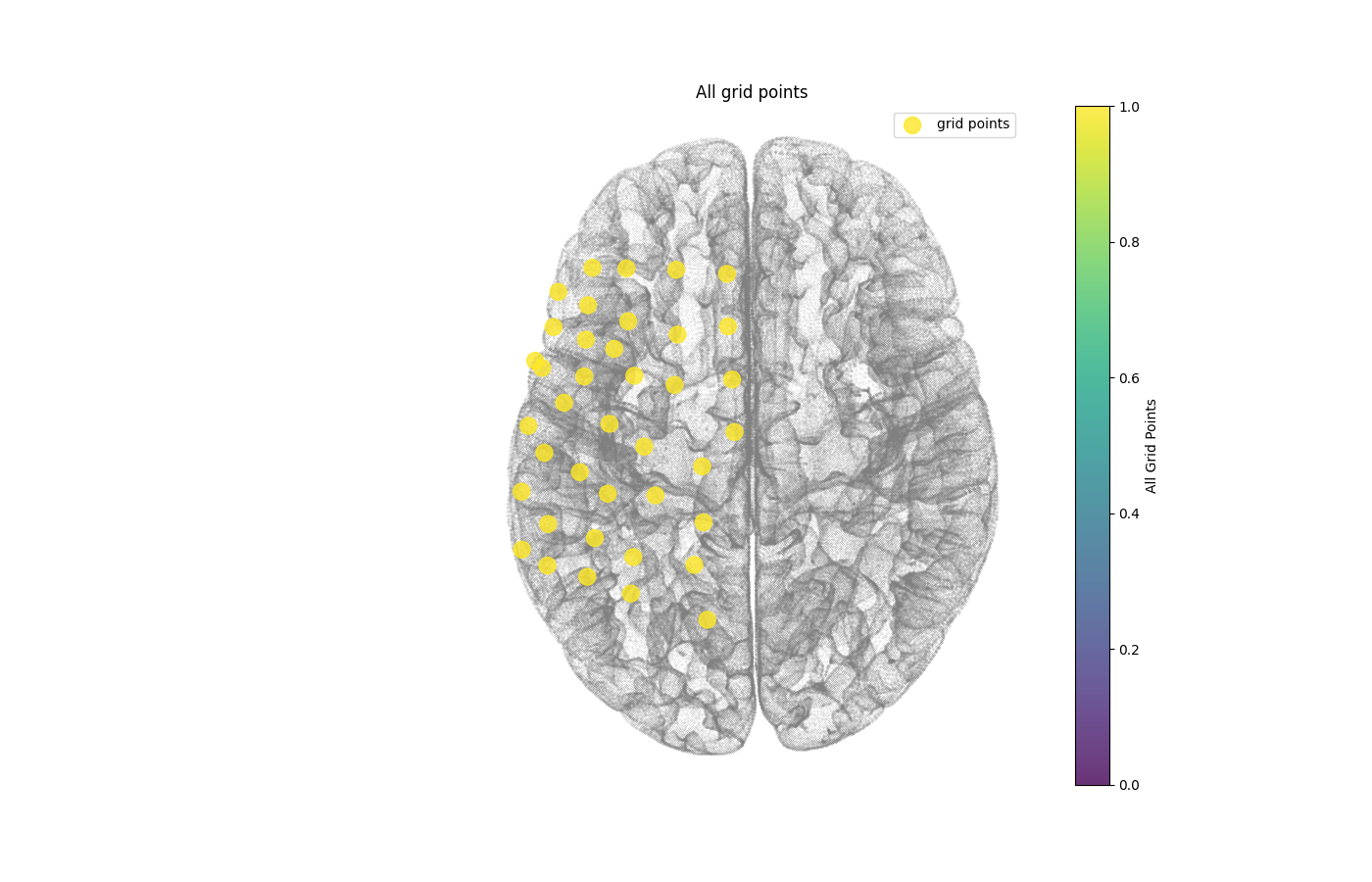
We can also plot only the ECoG electrodes or the grid points, with the help of the data saved in feature_reader.sidecar. BIDS sidecar files are json files where you store additional information, here it is used to save the ECoG strip positions and the grid coordinates, which are not part of the settings and channels.csv. We can check what is stored in the file and then use the nmplotter.plot_cortex function:

grid_plotter = nm.analysis.NM_Plot(
    ecog_strip=np.array(feature_reader.sidecar["coords"]["cortex_right"]["positions"]),
    grid_cortex=np.array(feature_reader.sidecar["grid_cortex"]),
    # grid_subcortex=np.array(feature_reader.sidecar["grid_subcortex"]),
    sess_right=feature_reader.sidecar["sess_right"],
    proj_matrix_cortex=np.array(feature_reader.sidecar["proj_matrix_cortex"]),
)

grid_plotter.plot_cortex(
    grid_color=np.sum(np.array(feature_reader.sidecar["proj_matrix_cortex"]), axis=1),
    lower_clim=0.0,
    upper_clim=1.0,
    cbar_label="Used Grid Points",
    title="ECoG electrodes projected onto cortical grid",
)

feature_reader.sidecar["coords"]["cortex_right"]["positions"]

[[37.318174, -48.61012664, 61.79765474], [40.1598943, -37.31592983, 64.31171618], [40.94303578, -27.21778456, 64.09518408], [39.78395522, -17.00523081, 63.86618136], [39.68813641, -5.528024572, 61.68254254], [37.51915924, 4.304913414, 60.54126355]]

feature_reader.nmplotter.plot_cortex(
    ecog_strip=np.array(
        feature_reader.sidecar["coords"]["cortex_right"]["positions"],
    ),
    lower_clim=0.0,
    upper_clim=1.0,
    cbar_label="Used ECoG Electrodes",
    title="Plot of ECoG electrodes",
)

feature_reader.nmplotter.plot_cortex(
    np.array(feature_reader.sidecar["grid_cortex"]),
    lower_clim=0.0,
    upper_clim=1.0,
    cbar_label="All Grid Points",
    title="All grid points",
)

The Projection Matrix

To go from the feature-channel matrix (n_features, n_channels) to the grid point matrix (n_features, n_gridpoints) we need a projection matrix that has the shape (n_channels, n_gridpoints). It maps the strengths of the signals in each ECoG channel to the correspondent ones in the cortical grid. In the cell below we plot this matrix, that has the property that the column sum over channels for each grid point is either 1 or 0.

plt.figure(figsize=(8, 5))
plt.imshow(np.array(feature_reader.sidecar["proj_matrix_cortex"]), aspect="auto")
plt.colorbar(label="Strength of ECoG signal in each grid point")
plt.xlabel("ECoG channels")
plt.ylabel("Grid points")
plt.title("Matrix mapping from ECoG to grid")

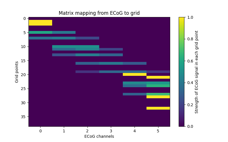
Text(0.5, 1.0, 'Matrix mapping from ECoG to grid')

Feature Plot in the Grid: An Example of Post-processing

First we take the dataframe with all the features in all time points.

df = feature_reader.feature_arr

df.iloc[:5, :5]

	LFP_RIGHT_0_LFP_RIGHT_2_fft_theta_mean	LFP_RIGHT_1_LFP_RIGHT_0_fft_theta_mean	LFP_RIGHT_2_LFP_RIGHT_1_fft_theta_mean	ECOG_RIGHT_0_avgref_fft_theta_mean	ECOG_RIGHT_1_avgref_fft_theta_mean
0	3.544938	3.462266	3.516675	3.784520	3.889221
1	-1.000000	1.000000	1.000000	-1.000000	1.000000
2	-0.640741	-0.660343	-1.106926	0.689275	0.758821
3	-0.226247	0.333361	-1.520981	1.322776	-0.454620
4	-0.370427	-0.840489	-0.320919	1.093448	-1.418237

Then we filter for only ‘avgref_fft_theta’, which gives us the value for fft_theta in all 6 ECoG channels over all time points. Then we take only the 6th time point - as an arbitrary choice.

fft_theta_oneTimePoint = np.asarray(
    df[df.columns[df.columns.str.contains(pat="avgref_fft_theta")]].iloc[5]
)
fft_theta_oneTimePoint

array([-0.35856691, -1.65213409,  0.67152411,  0.08666766,  0.74406089,
        1.17511129])

Then the projection of the features into the grid is gonna be the color of the grid points in the plot_cortex function. That is the matrix multiplication of the projection matrix of the cortex and 6 values for the fft_theta feature above.

grid_fft_Theta = (
    np.array(feature_reader.sidecar["proj_matrix_cortex"]) @ fft_theta_oneTimePoint
)

feature_reader.nmplotter.plot_cortex(
    np.array(feature_reader.sidecar["grid_cortex"]),
    grid_color=grid_fft_Theta,
    set_clim=True,
    lower_clim=min(grid_fft_Theta[grid_fft_Theta > 0]),
    upper_clim=max(grid_fft_Theta),
    cbar_label="FFT Theta Projection to Grid",
    title="FFT Theta Projection to Grid",
)

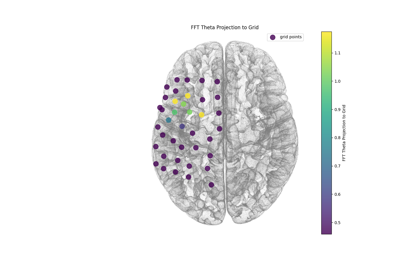
Lower and upper boundaries for clim were chosen to be the max and min values of the projection of the features (minimum value excluding zero). This can be checked in the cell below:

grid_fft_Theta

array([ 0.        , -0.35856691, -0.35856691,  0.        ,  0.        ,
       -0.88206403,  0.        , -0.6634492 ,  0.        ,  0.        ,
       -0.49283354, -0.25995071,  0.        , -0.10879517,  0.        ,
        0.        ,  0.45885887,  0.        ,  0.        ,  0.58028397,
        0.74406089,  1.17511129,  0.        ,  0.97422633,  1.01903534,
        0.        ,  0.        ,  1.03882634,  1.17511129,  0.        ,
        0.        ,  0.        ,  1.17511129,  0.        ,  0.        ,
        0.        ,  0.        ,  0.        ,  0.        ])

In the plot above we can see how the intensity of the fast fourier transform in the theta band varies for each grid point in the cortex, for one specific time point.