Note
Go to the end to download the full example code.
Analyzing temporal features#
Time series data can be characterized using oscillatory components, but assumptions of sinusoidality are for real data rarely fulfilled. See “Brain Oscillations and the Importance of Waveform Shape” Cole et al 2017 for a great motivation. We implemented here temporal characteristics based on individual trough and peak relations, based on the :meth:~`scipy.signal.find_peaks` method. The function parameter distance can be specified in the settings.yaml. Temporal features can be calculated twice for troughs and peaks. In the settings, this can be specified by setting estimate to true in detect_troughs and/or detect_peaks. A statistical measure (e.g. mean, max, median, var) can be defined as a resulting feature from the peak and trough estimates using the apply_estimator_between_peaks_and_troughs setting.
In py_neuromodulation the following characteristics are implemented:
Note
The nomenclature is written here for sharpwave troughs, but detection of peak characteristics can be computed in the same way.
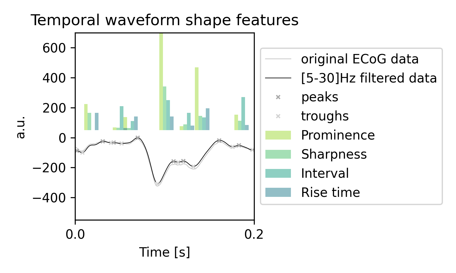
prominence: \(V_{prominence} = |\frac{V_{peak-left} + V_{peak-right}}{2}| - V_{trough}\)
sharpness: \(V_{sharpnesss} = \frac{(V_{trough} - V_{trough-5 ms}) + (V_{trough} - V_{trough+5 ms})}{2}\)
rise and decay rise time
rise and decay steepness
width (between left and right peaks)
interval (between troughs)
Additionally, different filter ranges can be parametrized using the filter_ranges_hz setting. Filtering is necessary to remove high frequent signal fluctuations, but limits also the true estimation of sharpness and prominence due to signal smoothing.
from typing import cast
import seaborn as sb
from matplotlib import pyplot as plt
from scipy import signal
from scipy.signal import fftconvolve
import numpy as np

import py_neuromodulation as nm
from py_neuromodulation import NMSettings
from py_neuromodulation.features import SharpwaveAnalyzer
We will first read the example ECoG data and plot the identified features on the filtered time series.
RUN_NAME, PATH_RUN, PATH_BIDS, PATH_OUT, datatype = nm.io.get_paths_example_data()

(
    raw,
    data,
    sfreq,
    line_noise,
    coord_list,
    coord_names,
) = nm.io.read_BIDS_data(PATH_RUN=PATH_RUN)
Extracting parameters from /opt/hostedtoolcache/Python/3.12.12/x64/lib/python3.12/site-packages/py_neuromodulation/data/sub-testsub/ses-EphysMedOff/ieeg/sub-testsub_ses-EphysMedOff_task-gripforce_run-0_ieeg.vhdr...
Setting channel info structure...
/opt/hostedtoolcache/Python/3.12.12/x64/lib/python3.12/site-packages/py_neuromodulation/utils/io.py:61: RuntimeWarning: Did not find any events.tsv associated with sub-testsub_ses-EphysMedOff_task-gripforce_run-0.

The search_str was "/opt/hostedtoolcache/Python/3.12.12/x64/lib/python3.12/site-packages/py_neuromodulation/data/sub-testsub/**/ieeg/sub-testsub_ses-EphysMedOff*events.tsv"
  raw_arr = read_raw_bids(bids_path)
Reading channel info from /opt/hostedtoolcache/Python/3.12.12/x64/lib/python3.12/site-packages/py_neuromodulation/data/sub-testsub/ses-EphysMedOff/ieeg/sub-testsub_ses-EphysMedOff_task-gripforce_run-0_channels.tsv.
/opt/hostedtoolcache/Python/3.12.12/x64/lib/python3.12/site-packages/py_neuromodulation/utils/io.py:61: RuntimeWarning: Other is not an MNE-Python coordinate frame for IEEG data and so will be set to 'unknown'
  raw_arr = read_raw_bids(bids_path)
Reading electrode coords from /opt/hostedtoolcache/Python/3.12.12/x64/lib/python3.12/site-packages/py_neuromodulation/data/sub-testsub/ses-EphysMedOff/ieeg/sub-testsub_ses-EphysMedOff_space-mni_electrodes.tsv.
/opt/hostedtoolcache/Python/3.12.12/x64/lib/python3.12/site-packages/py_neuromodulation/utils/io.py:61: RuntimeWarning: There are channels without locations (n/a) that are not marked as bad: ['MOV_RIGHT']
  raw_arr = read_raw_bids(bids_path)
/opt/hostedtoolcache/Python/3.12.12/x64/lib/python3.12/site-packages/py_neuromodulation/utils/io.py:61: RuntimeWarning: Not setting position of 1 misc channel found in montage:
['MOV_RIGHT']
Consider setting the channel types to be of EEG/sEEG/ECoG/DBS/fNIRS using inst.set_channel_types before calling inst.set_montage, or omit these channels when creating your montage.
  raw_arr = read_raw_bids(bids_path)
settings = NMSettings.get_fast_compute()

settings.features.fft = True
settings.features.bursts = False
settings.features.sharpwave_analysis = True
settings.features.coherence = False

settings.sharpwave_analysis_settings.estimator["mean"] = []
settings.sharpwave_analysis_settings.sharpwave_features.enable_all()
for sw_feature in settings.sharpwave_analysis_settings.sharpwave_features.list_all():
    settings.sharpwave_analysis_settings.estimator["mean"].append(sw_feature)

channels = nm.utils.set_channels(
    ch_names=raw.ch_names,
    ch_types=raw.get_channel_types(),
    reference="default",
    bads=raw.info["bads"],
    new_names="default",
    used_types=("ecog", "dbs", "seeg"),
    target_keywords=["MOV_RIGHT"],
)

stream = nm.Stream(
    sfreq=sfreq,
    channels=channels,
    settings=settings,
    line_noise=line_noise,
    coord_list=coord_list,
    coord_names=coord_names,
    verbose=False,
)
sw_analyzer = cast(
    SharpwaveAnalyzer, stream.data_processor.features.get_feature("sharpwave_analysis")
)
The plotted example time series, visualized on a short time scale, shows the relation of identified peaks, troughs, and estimated features:
data_plt = data[5, 1000:4000]

filtered_dat = fftconvolve(data_plt, sw_analyzer.list_filter[0][1], mode="same")

troughs = signal.find_peaks(-filtered_dat, distance=10)[0]
peaks = signal.find_peaks(filtered_dat, distance=5)[0]

sw_results = sw_analyzer.analyze_waveform(filtered_dat)

WIDTH = BAR_WIDTH = 4
BAR_OFFSET = 50
OFFSET_TIME_SERIES = -100
SCALE_TIMESERIES = 1

hue_colors = sb.color_palette("viridis_r", 6)

plt.figure(figsize=(5, 3), dpi=300)
plt.plot(
    OFFSET_TIME_SERIES + data_plt,
    color="gray",
    linewidth=0.5,
    alpha=0.5,
    label="original ECoG data",
)
plt.plot(
    OFFSET_TIME_SERIES + filtered_dat * SCALE_TIMESERIES,
    linewidth=0.5,
    color="black",
    label="[5-30]Hz filtered data",
)

plt.plot(
    peaks,
    OFFSET_TIME_SERIES + filtered_dat[peaks] * SCALE_TIMESERIES,
    "x",
    label="peaks",
    markersize=3,
    color="darkgray",
)
plt.plot(
    troughs,
    OFFSET_TIME_SERIES + filtered_dat[troughs] * SCALE_TIMESERIES,
    "x",
    label="troughs",
    markersize=3,
    color="lightgray",
)

plt.bar(
    troughs + BAR_WIDTH,
    np.array(sw_results["prominence"]) * 4,
    bottom=BAR_OFFSET,
    width=WIDTH,
    color=hue_colors[0],
    label="Prominence",
    alpha=0.5,
)
plt.bar(
    troughs + BAR_WIDTH * 2,
    -np.array(sw_results["sharpness"]) * 6,
    bottom=BAR_OFFSET,
    width=WIDTH,
    color=hue_colors[1],
    label="Sharpness",
    alpha=0.5,
)
plt.bar(
    troughs + BAR_WIDTH * 3,
    np.array(sw_results["interval"]) * 5,
    bottom=BAR_OFFSET,
    width=WIDTH,
    color=hue_colors[2],
    label="Interval",
    alpha=0.5,
)
plt.bar(
    troughs + BAR_WIDTH * 4,
    np.array(sw_results["rise_time"]) * 5,
    bottom=BAR_OFFSET,
    width=WIDTH,
    color=hue_colors[3],
    label="Rise time",
    alpha=0.5,
)

plt.xticks(
    np.arange(0, data_plt.shape[0], 200),
    np.round(np.arange(0, int(data_plt.shape[0] / 1000), 0.2), 2),
)
plt.xlabel("Time [s]")
plt.title("Temporal waveform shape features")
plt.legend(loc="center left", bbox_to_anchor=(1, 0.5))
plt.ylim(-550, 700)
plt.xlim(0, 200)
plt.ylabel("a.u.")
plt.tight_layout()

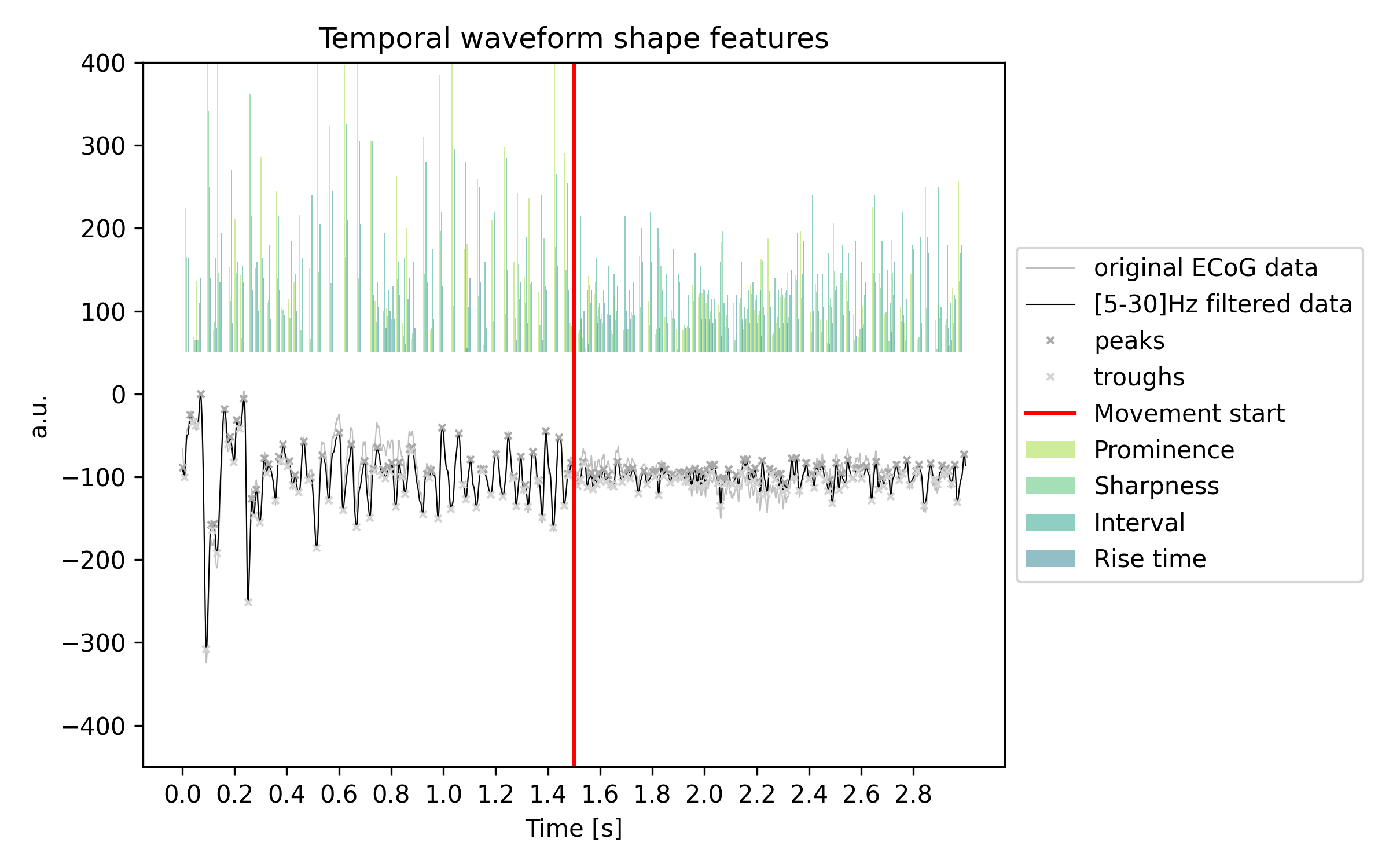
See in the following example a time series example, that is aligned to movement. With movement onset the prominence, sharpness, and interval features are reduced:
plt.figure(figsize=(8, 5), dpi=300)
plt.plot(
    OFFSET_TIME_SERIES + data_plt,
    color="gray",
    linewidth=0.5,
    alpha=0.5,
    label="original ECoG data",
)
plt.plot(
    OFFSET_TIME_SERIES + filtered_dat * SCALE_TIMESERIES,
    linewidth=0.5,
    color="black",
    label="[5-30]Hz filtered data",
)

plt.plot(
    peaks,
    OFFSET_TIME_SERIES + filtered_dat[peaks] * SCALE_TIMESERIES,
    "x",
    label="peaks",
    markersize=3,
    color="darkgray",
)
plt.plot(
    troughs,
    OFFSET_TIME_SERIES + filtered_dat[troughs] * SCALE_TIMESERIES,
    "x",
    label="troughs",
    markersize=3,
    color="lightgray",
)

plt.bar(
    troughs + BAR_WIDTH,
    np.array(sw_results["prominence"]) * 4,
    bottom=BAR_OFFSET,
    width=WIDTH,
    color=hue_colors[0],
    label="Prominence",
    alpha=0.5,
)
plt.bar(
    troughs + BAR_WIDTH * 2,
    -np.array(sw_results["sharpness"]) * 6,
    bottom=BAR_OFFSET,
    width=WIDTH,
    color=hue_colors[1],
    label="Sharpness",
    alpha=0.5,
)
plt.bar(
    troughs + BAR_WIDTH * 3,
    np.array(sw_results["interval"]) * 5,
    bottom=BAR_OFFSET,
    width=WIDTH,
    color=hue_colors[2],
    label="Interval",
    alpha=0.5,
)
plt.bar(
    troughs + BAR_WIDTH * 4,
    np.array(sw_results["rise_time"]) * 5,
    bottom=BAR_OFFSET,
    width=WIDTH,
    color=hue_colors[3],
    label="Rise time",
    alpha=0.5,
)

plt.axvline(x=1500, label="Movement start", color="red")

# plt.xticks(np.arange(0, 2000, 200), np.round(np.arange(0, 2, 0.2), 2))
plt.xticks(
    np.arange(0, data_plt.shape[0], 200),
    np.round(np.arange(0, int(data_plt.shape[0] / 1000), 0.2), 2),
)
plt.xlabel("Time [s]")
plt.title("Temporal waveform shape features")
plt.legend(loc="center left", bbox_to_anchor=(1, 0.5))
plt.ylim(-450, 400)
plt.ylabel("a.u.")
plt.tight_layout()

In the sharpwave_analysis_settings the estimator keyword further specifies which statistic is computed based on the individual features in one batch. The “global” setting segment_length_features_ms specifies the time duration for feature computation. Since there can be a different number of identified waveform shape features for different batches (i.e. different number of peaks/troughs), taking a statistical measure (e.g. the maximum or mean) will be necessary for feature comparison.
Example time series computation for movement decoding#
We will now read the ECoG example/data and investigate if samples differ across movement states. Therefore we compute features and enable the default sharpwave features.
settings = NMSettings.get_default().reset()

settings.features.sharpwave_analysis = True
settings.sharpwave_analysis_settings.filter_ranges_hz = [[5, 80]]

channels["used"] = 0  # set only two ECoG channels for faster computation to true
channels.loc[[3, 8], "used"] = 1

stream = nm.Stream(
    sfreq=sfreq,
    channels=channels,
    settings=settings,
    line_noise=line_noise,
    coord_list=coord_list,
    coord_names=coord_names,
    verbose=True,
)

df_features = stream.run(data=data[:, :30000], save_csv=False)
/opt/hostedtoolcache/Python/3.12.12/x64/lib/python3.12/site-packages/pydantic/main.py:464: UserWarning: Pydantic serializer warnings:
  PydanticSerializationUnexpectedValue(Expected `FrequencyRange` - serialized value may not be as expected [field_name='filter_ranges_hz', input_value=[5, 80], input_type=list])
  return self.__pydantic_serializer__.to_python(
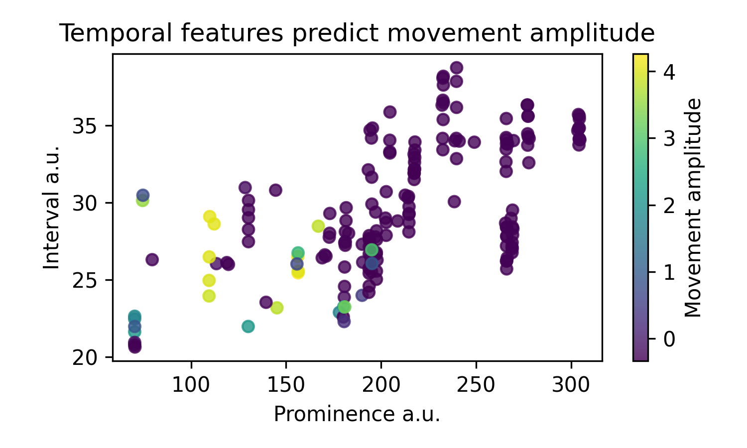
We can then plot two exemplary features, prominence and interval, and see that the movement amplitude can be clustered with those two features alone:
plt.figure(figsize=(5, 3), dpi=300)
print(df_features.columns)
plt.scatter(
    df_features["ECOG_RIGHT_0_avgref_Sharpwave_Max_prominence_range_5_80"],
    df_features["ECOG_RIGHT_5_avgref_Sharpwave_Mean_interval_range_5_80"],
    c=df_features.MOV_RIGHT,
    alpha=0.8,
    s=30,
)
cbar = plt.colorbar()
cbar.set_label("Movement amplitude")
plt.xlabel("Prominence a.u.")
plt.ylabel("Interval a.u.")
plt.title("Temporal features predict movement amplitude")
plt.tight_layout()

Index(['ECOG_RIGHT_0_avgref_Sharpwave_Max_prominence_range_5_80',
       'ECOG_RIGHT_0_avgref_Sharpwave_Mean_interval_range_5_80',
       'ECOG_RIGHT_0_avgref_Sharpwave_Max_sharpness_range_5_80',
       'ECOG_RIGHT_5_avgref_Sharpwave_Max_prominence_range_5_80',
       'ECOG_RIGHT_5_avgref_Sharpwave_Mean_interval_range_5_80',
       'ECOG_RIGHT_5_avgref_Sharpwave_Max_sharpness_range_5_80', 'time',
       'MOV_RIGHT'],
      dtype='str')
Total running time of the script: (0 minutes 1.656 seconds)